

For many of us, the deep sea is a bit of a mystery. But an exciting interactive digital tool at the National Museum of the Royal Navy is bringing the seabed to life!
It turns out that the sea floor is just as interesting as the land where we spend most of our time (unless you’re a crab, of course, in which case you spend most of your time on the sea floor). I recently learnt about the sea floor at the National Museum of the Royal Navy in Portsmouth, in their “Worlds Beneath the Waves” exhibition, which documents 150-years of deep-sea exploration.
One ship which revolutionised deep ocean study was HMS Challenger. It left London in 1858 and went on to make a 68,890 nautical-mile journey all over the earth’s oceans. One of its scientific goals was to measure the depth of the seabed as it circled the earth. To make these measurements, a long rope with a weight at one end was dropped into the water, which sank to the bottom. The length of the rope needed until the weight hit the floor was measured. It’s a simple process, but it worked!
Thankfully, modern technology has caught up with bathymetry (the study of the sea floor). Now, sea floor depths are measured using sonar (so sound) and lidar (light) from ships or using special sensors on satellites. All of these methods send signals down to the seabed, and count how long it takes for a response. Knowing the speed of sound or light through air and water, you can calculate the distance to whatever reflected the signal.
You may be thinking, why do we need to know how deep the ocean is? Well, apart from the human desire to explore and mapour planet, it’s also useful for navigation and safety: in smaller waterways and ports, it’s very helpful to know whether there’s enough water below the boat to stay afloat!
It’s also useful to look at fault lines, the deep valleys (such as Challenger Deep, the deepest known point in the ocean, named after HMS Challenger), and underwater mountain ranges which separate continental plates. Studying these can help us to predict earthquakes and understand continental drift (read more about continental drift).
We now have a much better understanding of the seabed, including detailed maps of sea floor topography around the world. So, we know what the ocean floor looks like at the moment, but how can we use this to understand the future of our waterways? This is where computers come in.
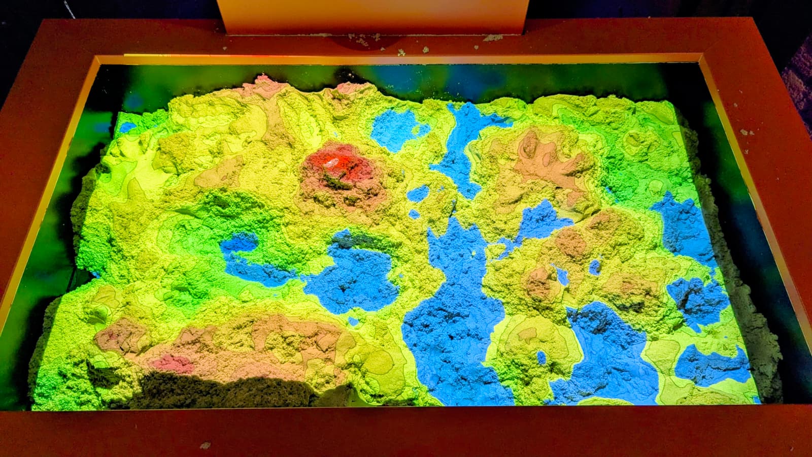
Near the end of the exhibition sits a table covered in sand, which has, projected onto it, the current topography of the sand. Where the sand is piled up higher is coloured red and orange, and lower in green and blue. Looking across the table you can see how sand at the same level, even far apart, is still within the same band of colour.
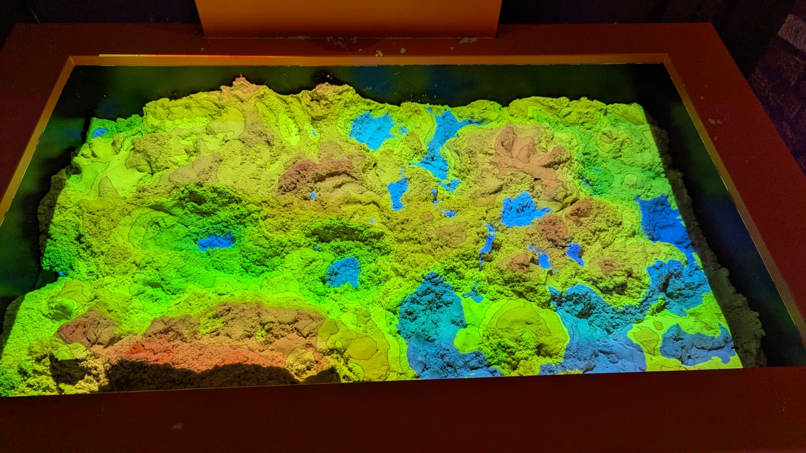
But this isn’t even the coolest part! When you pick up and move sand around, the colours automatically adjust to the new sand topography, allowing you to shape the seabed at will. The sand itself, however, will flow and move depending on gravity, so an unrealistically tall tower will soon fall down and form a more rotund mound.
Want to know what will happen if a meteor impacts? Grab a handful of sand and drop it onto the table (without making a mess) and see how the topographical map changes with time!
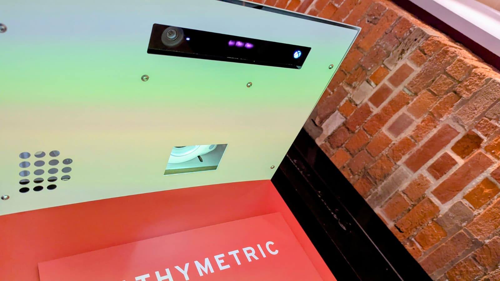
So how does this work? Looking above the table, you can see an Xbox Kinect sensor, and a projector. The Kinect works much like the lidar systems installed on ships – it sends beams of infrared lights down onto the sand, which bounce off back to the sensor in a measured time. This creates a depth map, just like ships do, but on a much smaller scale. This map is turned into colours and projected back on to the sand.

This is not the only feature of this table, however: it can also run physics simulations! By placing your hand over the sand, you can add virtual water, which flows realistically into the lower areas of sand, and even responds to the movement of sand.
The mixing of physical and digital representations of data like this is an example of augmented, or mixed, reality. It can help visualise things that you might otherwise find difficult to imagine, perhaps by simulating the effects of building a new dam, for example. Models like this can help experts and students, and, indeed, museum visitors, to see a problem in a different and more interactive way.
– Daniel Gill, Queen Mary University of London
More on…
- Continental drift
- Jet-propelled creatures of the oceans!
- Data Visualisation and Sonification (CS4FN Portal)
- Worlds Between the Waves Exhibition [EXTERNAL]
Subscribe to be notified whenever we publish a new post to the CS4FN blog.
This blog is funded by EPSRC on research agreement EP/W033615/1.


